This is Part 3. Follow links for Part 1, 2, 4, 5, 6, 7 and 8.
In Part 1, we showed that a simple “VT and chill” strategy can come with a hidden structural cost. In this article, we go one step further by examining where that cost comes from and whether investors can capture it. Using decades of historical data, we’ll compare regional allocation approaches, quantify their impact on return and explore why small portfolio policy changes can compound into meaningful differences over a lifetime.
Data Calibration Test
Before comparing portfolio outcomes, the first step we did was to verify that the data accurately reproduces a global market-cap weighted portfolio.
To test this, we compared:
- P1: VT-style continuous market-weight portfolio
- With the annual market-weight rebalanced VTSAX + VTIAX portfolio
From 1970 through 2025:
| Portfolio | CAGR |
|---|---|
| VT (P1) | 9.3604% |
| Annual Market Weight Rebalance (VTSAX + VTIAX) | 9.4958% |
The annualized difference: +0.1238% per year. Correlation: 99.7562%
The correlation is effectively perfect. The small return difference is expected because annual rebalancing only approximates the continuous market-weight adjustments that occur naturally inside VT.
This confirms that the historical data used in our portfolio construction methodology is consistent. The performance differences observed later cannot be dismissed as data artifacts.
Test plan
- For 60/40 US/International
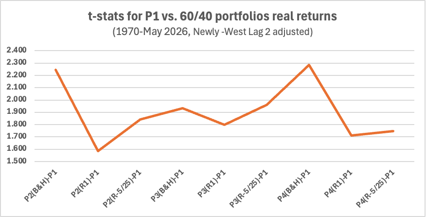
- Compute Newly-West Lag 2 adjusted t-stats between the real returns of the benchmark 60/40 portfolios, P2,3 and 4 in B&H, R1 and R-5/25 configurations, and P1.
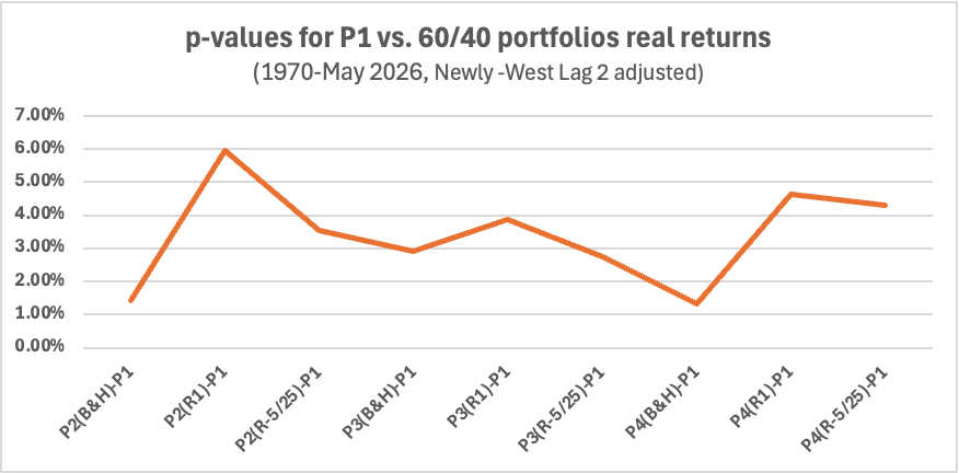
- Compute the corresponding p-values for the above t-stats.
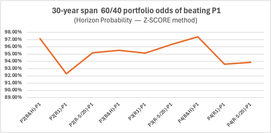
- Compute 30 year horizon probability that the benchmark portfolios will have higher real returns than P1 using the Z-score method.
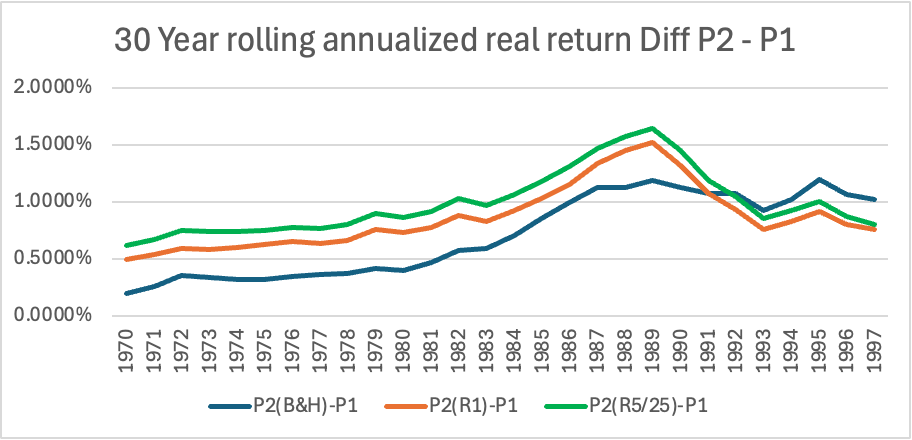
- Compute the actual 30 year rolling real return difference between the benchmark portfolios and P1.
- Compute P2(B&H) vs P1 for 30 year rolling real returns starting with start year’s VT weights.
Short recap:
- Portfolio composition:
- P1: VT: 100
- P2: VTSAX/VTIAX 60/40
- P3: VTSAX/VTMGX/VEMAX 60/32/8
- P4: VTSAX/VEUSX/VPADX/VEMAX 60/20/12/8
- Rebalancing:
- B&H: buy and hold
- R1: rebalance every year
- R-5/25: Rebalance using 5% absolute or 25% relative thresholds.
Full period 1970-2026 statistics
A t-statistic (t-stat) measures how far your observed result is from what you’d expect by random chance, expressed in units of standard error. The Newey-West adjustment corrects for the fact that returns aren’t independent year-to-year (good years tend to follow good years).
For 57 samples a t-stat value of 1.673 indicates a 5% chance that the result is due to chance.
We are doing what is called a one-tailed test specifically testing whether slice portfolios outperform VT. A p-value is the probability of observing our results if there were actually no real effect and only random chance was at work.
The Z-score method calculates the mathematical probability of outperformance over a 30-year horizon assuming returns follow a normal distribution. The Z-score odds are a reasonable heuristic, but the 30-year rolling results, in next section, is the more trustworthy evidence. The two are broadly consistent, which is reassuring.
| Portfolio | yearly t-stat (NW-Lag2) | p-value | 30 year odds > P1 (Z-score method) |
|---|---|---|---|
| P2(B&H)-P1 | 2.245 | 1.44% | 97.16% |
| P2(R1)-P1 | 1.583 | 5.95% | 92.29% |
| P2(R-5/25)-P1 | 1.841 | 3.54% | 95.19% |
| P3(B&H)-P1 | 1.932 | 2.92% | 95.53% |
| P3(R1)-P1 | 1.797 | 3.89% | 95.15% |
| P3(R-5/25)-P1 | 1.960 | 2.75% | 96.34% |
| P4(B&H)-P1 | 2.284 | 1.31% | 97.40% |
| P4(R1)-P1 | 1.710 | 4.64% | 93.62% |
| P4(R-5/25)-P1 | 1.747 | 4.30% | 93.88% |
30-Year Rolling Period Results (60/40)
The 30-year analysis is even more compelling. Twenty-eight separate 30-year rolling periods were evaluated across every portfolio specification:
- Average annual advantage ranged from 0.75% to 1.45%
- Median results closely matched averages
- Minimum observations remained positive in all cases
The persistence of the advantage over three decades is difficult to dismiss as random variation.
| count = 28 | P2(B&H)-P1 | P2(R1)-P1 | P2(R5/25)-P1 |
| min | 0.2014% | 0.4943% | 0.6213% |
| max | 1.1991% | 1.5214% | 1.6439% |
| average | 0.7073% | 0.8623% | 0.9878% |
| stdev | 0.3516% | 0.2762% | 0.2770% |
| median | 0.6512% | 0.7888% | 0.9077% |
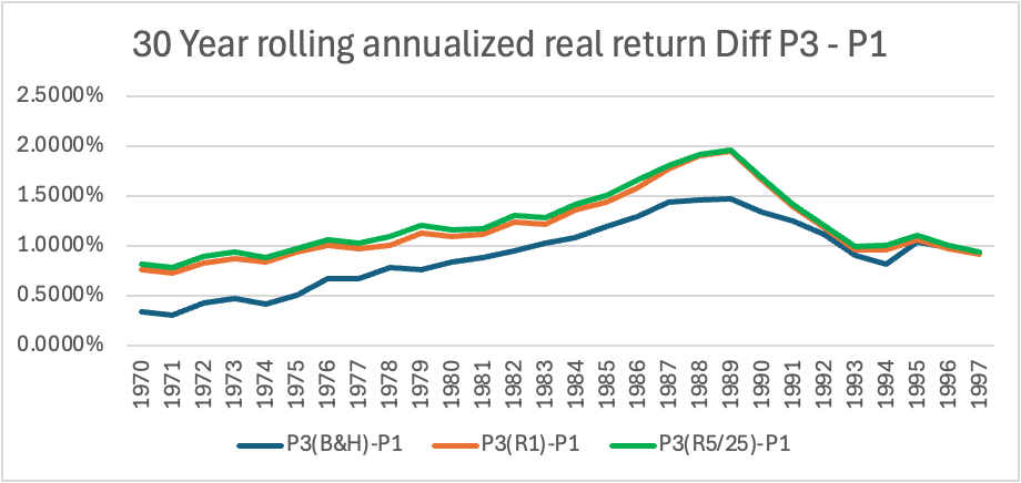
| count = 28 | P3(B&H)-P1 | P3(R1)-P1 | P3(R5/25)-P1 |
| min | 0.2988% | 0.7297% | 0.7863% |
| max | 1.4741% | 1.9459% | 1.9582% |
| average | 0.9042% | 1.1722% | 1.2205% |
| stdev | 0.3450% | 0.3373% | 0.3295% |
| median | 0.9129% | 1.0785% | 1.1300% |
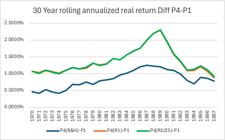
| count = 28 | P4(B&H)-P1 | P4(R1)-P1 | P4(R5/25)-P1 |
| min | 0.4200% | 0.8771% | 0.9134% |
| max | 1.2532% | 2.2917% | 2.3000% |
| average | 0.8292% | 1.3654% | 1.3715% |
| stdev | 0.2588% | 0.3699% | 0.3706% |
| median | 0.8056% | 1.2286% | 1.2400% |
The directional conclusion is robust: the slice premium has been remarkably persistent over 30-year horizons, and the Z-score method, with it’s limitations, is not creating a phantom result. The rolling 30 year window data confirms that independently.
P2(B&H) vs. P1 30 year annualized rolling real return difference when starting at VT weights.
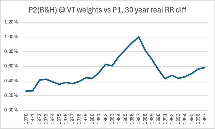
| count = 28 | P2(B&H)-P1 (30 Y RR starting @VT weights) |
|---|---|
| min | 0.2654% |
| max | 1.0007% |
| average | 0.5329% |
| stdev | 0.1881% |
| median | 0.4679% |
Here we wanted to do an apples-to-apples comparison and for every 30 year period P2 started with the same weights as VT. The results are unexpectedly positive. P2 won every time.
Statistical Significance
We chose to run the analysis on the yearly return difference because there was not enough yearly data to statistically analyze N=30 or even N=20 year return differences. We needed 4xN sample size for that.
To determine the significance of the return difference, we run a time-series Ordinary Least Squares (OLS) regression with Newey-West 2 year lag corrections to penalize any multi-year economic trends (autocorrelation).
The one year real return statistics show that for 8 out of 9 60/40 benchmark portfolios we have an adjusted t-stat derived p-value < 5%. The probability that the results are due to pure chance is less than 5%. In the one exception case the p-value was 5.92%.
This shows that while navigating the short-term year-to-year noise of custom slicing can be tricky, the long-term compounding odds are overwhelmingly stacked in your favor if you step away from market-cap weighting.
A Possible Risk-Based Explanation
A natural question is: if regional-slice portfolios historically outperformed VT, why should that premium exist at all?
One possible answer is that investors in VT are purchasing a form of insurance.
A market-cap weighted portfolio continuously updates its holdings to reflect the market’s collective judgment about the future. As regions grow in economic importance and market capitalization, VT automatically increases exposure. As regions shrink, VT reduces exposure. In effect, investors are outsourcing the problem of forecasting the future to the market itself.
Regional-slice portfolios take a different approach. By maintaining fixed regional allocations or rebalancing back to predetermined targets, investors are implicitly making an active bet that today’s market-cap weights may not perfectly predict tomorrow’s winners. They are willing to tolerate larger deviations from the global market portfolio in exchange for the possibility of capturing a rebalancing premium, a mean-reversion effect, or a momentum effect.
Historically, that willingness was rewarded. But the reward was not free.
The risk is that future economic leadership may undergo a permanent structural shift that market-cap weights correctly anticipate and regional-slice portfolios fail to recognize. In that scenario, VT’s continuous adaptation would be an advantage rather than a drag.
Viewed through this lens, the historical premium documented in this series may not represent a free lunch. Instead, it may be compensation for accepting the risk that the future will look very different from the past.
An Alternative Explanation: The Equity Issuance Effect
Another possible explanation involves the way market-cap weighted portfolios respond to new equity issuance.
When companies issue new shares, the supply of equity increases. Because market-cap weighted funds allocate capital based on market capitalization, they automatically direct additional capital toward regions and companies that have expanded their equity base.
This mechanism helps channel capital to growing firms and economies, which is one of the strengths of market-cap weighting. However, it also means that VT investors systematically absorb a large share of new equity issuance.
A regional-slice portfolio is less sensitive to these flows. Its allocation is determined primarily by regional targets rather than by changes in the global supply of publicly traded equity.
As a result, regional-slice investors may avoid some of the dilution associated with persistent net share issuance while still benefiting from the economic growth generated by the capital that newly issued equity helps finance.
Viewed from this perspective, part of the historical return gap may represent compensation earned by investors who were less willing to continuously fund the expansion of the global equity supply.
Whether this effect is large enough to explain a meaningful portion of the observed premium remains an open question, but it provides another potential mechanism linking portfolio construction rules to long-term returns.
Conclusion
The calibration test confirmed that the historical data accurately reproduces a global market-cap weighted portfolio, giving confidence that the performance differences observed throughout this analysis are not artifacts of the dataset or portfolio construction methodology.
Across every portfolio tested, regional-slice portfolios outperformed the continuously market-cap weighted benchmark. The advantage persisted under buy-and-hold, annual rebalancing, and 5/25 threshold rebalancing, and remained statistically significant in 8 of the 9 portfolio configurations after applying Newey-West autocorrelation adjustments.
Perhaps even more compelling, the advantage was remarkably consistent over long investment horizons. Across twenty-eight 30-year rolling periods, every benchmark portfolio produced positive average excess returns over VT, with no evidence that the historical premium was driven by a small number of exceptional decades.
None of this proves that regional-slice portfolios will outperform VT in the future. Markets evolve, and the historical relationship may not persist indefinitely.
What the evidence does suggest, however, is that the return premium documented in Parts 1 through 3 is unlikely to be a statistical accident. It appears to arise from a structural difference in portfolio construction.
A continuously market-cap weighted portfolio like VT systematically increases exposure to regions that have recently become larger while reducing exposure to those that have become smaller. Regional-slice portfolios deliberately break that feedback loop. Depending on the implementation, they capture some combination of a contrarian rebalancing premium, a momentum effect, or both, while accepting the possibility that market-cap weighting may better adapt to future structural shifts.
CONTINUE TO PART 4 ->
Disclaimer: This blog post is for informational purposes only and should not be considered financial advice. Consult with a qualified financial advisor for personalized guidance.
Leave a Reply